Bootstrap the RMST (restricted mean survival time) with option for automatic group merging
R function for AJCC Evidence Based Core, 2020.
Nonparametric ROC Analysis
Some of my R and S-PLUS functions for nonparametric analysis of ordinal categorical data (especially useful for analyzing data from diagnostic studies).
roc curves (R software for plotting roc curves)
multivariate roc data (S-PLUS software for tests on multirater data)
Bayesian Nonparametric Maximum Likelihood Estimator for Mixture Models
Blocked Gibbs sampler for finite normal mixture model in which the mean and variance are derived from an unknown mixture distribution with a finite (but unknown) number of components. Runs under R.
Uses two different approximations for the Dirichlet process:
(1) Stick Breaking Truncation
(2) Weak Limit Finite Dimensional Prior
Note that (2) is a nice way to put an upper bound on the number of mixture components (see Ishwaran, James and Sun, 2001; also see Example 1 below).
References
Ishwaran, H. and Zarepour, M. (2000). Markov chain Monte Carlo in approximate Dirichlet and beta two-parameter process hierarchical models. Biometrika, 87, 371-390. pdf
Ishwaran, H. and James, L.F. (2001). Gibbs sampling methods for stick-breaking priors. J. Amer. Stat. Assoc. 96, 161-173. pdf
Ishwaran, H., James, L.F. and Sun, J. (2001). Bayesian model selection in finite mixtures by marginal density decompositions. J. Amer. Stat. Assoc. 96, 1316-1332. pdf
Ishwaran, H. and James, L.F. (2002). Approximate Dirichlet process computing in finite normal mixtures: smoothing and prior information. J. Comp. Graph. Statist. 11, 508-532. pdf
Installation for Unix, Linux and OS-X
Download the R program ("normalMixture.1.2.R") and the C interface ("bayesian.c"). Then type
R CMD SHLIB bayesian.c
in the directory where you've place the two files. Start up R and simply type the following two commands before running the program:
source("normalMixture.1.2.R")
dyn.load("bayesian.so")
Example 1 (Finding the Bayesian NPMLE: Two Different Approaches)
Data consists of measurements of Sodium-Lithium Countertransport (SLC) on 190 individuals. It is believed that SLC measurements are derived from one of two competing genetic models: simple dominance, or additive. In the simple dominance model there are 2 alleles A1 and A2 and they form two phenotypes (A1A1 and A1A2) and (A2A2). In the additive model the two alleles form 3 phenotypes (A1A1), (A1A2) and (A2A2). Thus the simple dominance model corresponds to a 2-point mixture and the additive model to a 3-point mixture. We would like to find out which is the true model. See Roeder, K. (1994), "A graphical technique for determining the number of components in a mixture of normals". J. of the Amer. Statist. Assoc. 89, 487-495.
x=10*c(
.467,.430,.192,.192,.293,.160,.164,.126,.328,.202,.282,.328,.247,.132,
.138,.224,.512,.221,.252,.193,.236,.186,.346,.219,.177,.349,.272,.245,
.213,.197,.229,.245,.210,.281,.175,.273,.439,.471,.451,.237,.313,.136,
.245,.391,.349,.158,.252,.416,.232,.183,.254,.195,.141,.151,.073,.300,
.231,.075,.208,.267,.187,.244,.245,.231,.167,.337,.251,.209,.181,.411,
.191,.288,.280,.119,.394,.443,.423,.534,.393,.273,.149,.225,.159,.170,
.329,.183,.262,.250,.179,.329,.253,.270,.310,.321,.333,.284,.380,.222,
.178,.265,.289,.199,.309,.279,.194,.203,.139,.162,.251,.619,.343,.155,
.340,.332,.412,.218,.304,.261,.206,.231,.182,.267,.198,.191,.258,.179,
.197,.188,.202,.150,.201,.255,.293,.255,.189,.414,.292,.253,.168,.295,
.215,.213,.267,.216,.264,.138,.239,.288,.311,.414,.462,.361,.623,.199,
.215,.321,.273,.259,.206,.376,.228,.155,.186,.097,.176,.174,.386,.393,
.198,.243,.326,.250,.590,.461,.361,.321,.236,.139,.316,.313,.263,.180,
.184,.354,.264,.269,.171,.359,.338,.163)
Roeder (1994) argued that the variances are equal in this problem. Therefore, we use the equalVar=T option. Because of the large number of iterations used (needed to find the NPMLE) we turn off verbose details. This suppresses dynamic information like number of iterations completed. Here is the call to normalMixture:
set.seed(1)
normalMixture(x,n.iter1=2000,n.iter2=25000,equalVar=T,verbose.flag=F)
The output is:
$mean
[1] 2.228980 3.835631 5.998110
$var
[1] 0.3311933 0.3311933 0.3311933
$prob
[1] 0.7827038 0.1996390 0.0176562
$loglik
[1] -255.4526
The mean, var and prob give the Bayesian NPMLE. The loglik is the penalized log-likelihood value.
The analysis reveals the presence of 3 mixture components for the mean (2.2, 3.8 and 5.9) and the value for the variance is roughly 0.33. The additive model is the most likely scenario here reflecting the evidence of a 3-point mean mixture model.
The preceding analysis was based on infinite dimensional prior. Let's consider what happens if we use a prior whose number of components N is bounded by the underlying biology. Here we set N=3. To call the finite dimensional prior we set the option stickBreak=F.
We use the same seed value as before to make the comparison as close as possible. Here is the new call:
set.seed(1)
normalMixture(x,n.iter1=2000,n.iter2=25000,equalVar=T,stickBreak=F,N=3,verbose.flag=F)
The output is:
$mean
[1] 2.233603 3.806356 5.740366
$var
[1] 0.3359349 0.3359349 0.3359349
$prob
[1] 0.77861661 0.20088694 0.02049645
$loglik
[1] -255.2673
The results are almost identical to our previous values. Only one small difference is that the penalized log-likelihood is slightly smaller. This reflects a slight improvement in the analysis by taking into account the underlying science. In combination with our previous analysis the results provide compelling evidence of a 3-component mixture model.
Example 2 (Finding the Bayesian NPMLE: equal and unequal variances)
Here the data are velocities in km/sec of 82 galaxies from 6 well-separated conic sections of an 'unfilled' survey of the Corona Borealis region. Multimodality in such surveys is evidence for voids and superclusters in the far universe. See Roeder, K. (1990), "Density estimation with confidence sets exemplified by superclusters and voids in galaxies". J. Amer. Statist. Assoc. 85, 617-624.
x <- c(
9172, 9350, 9483, 9558, 9775, 10227, 10406, 16084,
16170, 18419, 18552, 18600, 18927, 19052, 19070, 19330,
19343, 19349, 19440, 19473, 19529, 19541, 19547, 19663,
19846, 19856, 19863, 19914, 19918, 19973, 19989, 20166,
20175, 20179, 20196, 20215, 20221, 20415, 20629, 20795,
20821, 20846, 20875, 20986, 21137, 21492, 21701, 21814,
21921, 21960, 22185, 22209, 22242, 22249, 22314, 22374,
22495, 22746, 22747, 22888, 22914, 23206, 23241, 23263,
23484, 23538, 23542, 23666, 23706, 23711, 24129, 24285,
24289, 24366, 24717, 24990, 25633, 26690, 26995, 32065,
32789, 34279)
(A) First we find the NPMLE assuming an equal variance model:
set.seed(1)
normalMixture(x,n.iter1=2000,n.iter2=25000,equalVar=T,verbose.flag=F)
The ouput yields a 3-component mixture:
| $mean | 21396.251 | 9476.683 | 32995.854 |
| $prob | 0.88502649 | 0.08484509 | 0.02983183 |
(B) Next, let's try an unequal variance model:
set.seed(1)
normalMixture(x,n.iter1=2000,n.iter2=25000,verbose.flag=F)
The ouput once again yields a 3-component mixture model:
| $mean | 21189.64 | 9950.36 | 31221.10 |
| $var | 5377921 | 2112348 | 15805307 |
| $prob | 0.83211849 | 0.11342191 | 0.05314351 |
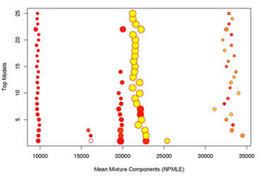
(C) Finally let's try an unequal variance model, using a flat prior for the variance:
set.seed(1)
normalMixture(x,n.iter1=2000,n.iter2=25000,tauTrunc=T,verbose.flag=F,file.out="galaxy")
Now we find a 5 component mixture model:
| $mean | 9776.947 | 22825.921 | 25382.718 | 19747.474 | 16159.313 |
| $var | 341143.91 | 1650104.91 | 19507389.04 | 426082.41 | 8711.43 |
| $prob | 0.06071068 | 0.34265300 | 0.17407575 | 0.38632544 | 0.02460401 |
If we check "galaxy.pdf" for the graphical summary, we see that the top 25 models oscillate from 3-5 mixtures. The 3-component models look similar to the NPMLE found in (B).